k.
Non stationary time series
Most
economic (and also many other) time series do not satisfy the
stationarity conditions stated earlier for which ARMA models have
been derived. Then these times series are called non
stationary and should be re-expressed such that they become
stationary with respect to the variance and the mean.
It
is not suggested that the description of the following re-expression
tools is exhaustive! They rather form a set of tools which have
shown to be useful in practice. It is quite evident that many
extensions are possible with respect to re-expression tools: these
are discussed in literature such as in JENKINS (1976 and 1978),
MILLS (1990), MCLEOD (1983), etc...
Transformation
of time series
If
we write a time series as the sum of a deterministic mean and a
disturbance term
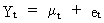
(V.I.1-193)

(V.I.1-194)
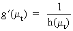
where
h is an arbitrary function.

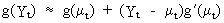
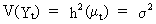
(V.I.1-195)
This
can be used to obtain the variance of the transformed series
(V.I.1-196)
which
implies that the variance can be stabilized by imposing
(V.I.1-197)
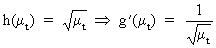
Accordingly,
if the standard deviation of the series is proportional to the mean
level

(V.I.1-198)
then
(V.I.1-199)
from
which it follows that

(V.I.1-200)
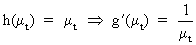
In
case the variance of the series is proportional to the mean level,
then
(V.I.1-201)
from
which it follows that

(V.I.1-202)
With
the use of a Standard
Deviation / Mean Procedure (SMP) we are able to detect heteroskedasticity in the time series. Above that, with the help of
the SMP, it is quite often possible to find an appropriate
transformation which will ensure the time series to be
homoskedastic. In fact, it is assumed that there exists a
relationship between the mean level of the time series and the
variance or standard deviation as in

(V.I.1-203)
which
is an explicitly assumed relationship, in contrast to (V.I.1-194).
The
SMP is generated by a three step process:
 |
the
time series is spilt into equal (chronological) segments; | |
|
for
each segment the arithmetic mean and standard deviation is
computed; | |
|
the
mean and S.D. of each segment is plotted or regressed against
each other. | |
By
selecting the length of the segments equal to the seasonal period
one ensures that the S.D. and mean is independent from the seasonal
period.
In
practice one of the following patterns will be recognized (as
summarized in the graph). Note that the lambda parameter should take
a value of zero when a linearly proportional association between
S.D. and the mean is recognized.
The
value of lambda is in fact the transformation parameter which
implies the following:
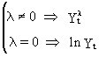
(V.I.1-204)
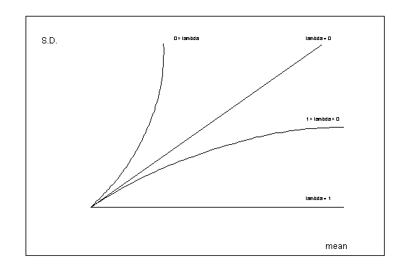
(Figure
V.I.1-10)
Differencing
of time series
With
the use of the Autocorrelation
Function (ACF) (with autocorrelations on the y axis and the
different time lags on the x axis) it is possible to detect unstationarity
of the time series with respect to the mean
level.
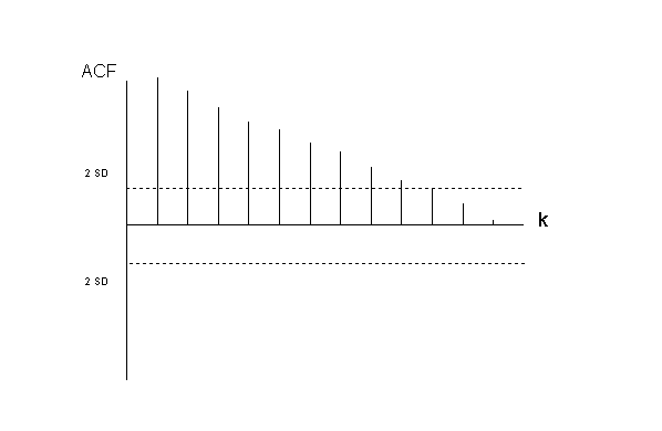
(figure
V.I.1-11)
When
the ACF of the time series is slowly
decreasing, this is an indication that the mean is not
stationary. An example of such an ACF is given in figure (V.I.1-11).
The
differencing operator (nabla) is used to make the time series
stationary. |