Time Series Analysis - ARIMA models - AR(2) process

c. The AR(2) process

The AR(2) process is defined as

(V.I.1-94)

where W_t is a stationary time series, e_t is a white noise error term, and F_t is the forecasting function.

The process defined in (V.I.1-94) can be written in the form

(V.I.1-95)

and therefore

(V.I.1-96)

Now, for (V.I.1-96) to be valid, it easily follows that

(V.I.1-97)

and that

(V.I.1-98)

and that

(V.I.1-99)

and finally that

(V.I.1-100)

The model is stationary if the y_i weights converge. This is the case when some conditions on f₁ and f₂ are imposed. These conditions can be found on using the solutions of the polynomial of the AR(2) model. The so-called characteristic equation is used to find these solutions

(V.I.1-101)

The solutions of x₁ and x₂ are

(V.I.1-102)

which can be either real or complex. Notice that the roots are complex if

When these solutions, in absolute value, are smaller than 1, the AR(2) model is stationary.

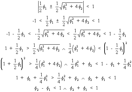
Later, it will be shown that these conditions are satisfied if f₁ and f₂ lie in a (Stralkowski) triangular region restricted by

(V.I.1-103)

The derivation of the theoretical ACF and PACF for an AR(2) model is described below.

On multiplying the AR(2) model by W_t-k, and taking expectations we obtain

(V.I.1-104)

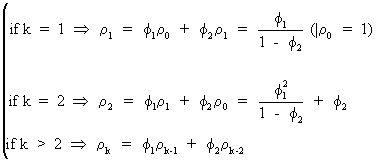
From (V.I.1-97) and (V.I.1-98) it follows that

(V.I.1-105)

Now it is possible to combine (V.I.1-104) with (V.I.1-105) such that

(V.I.1-106)

from which it follows that

(V.I.1-107)

Therefore

(V.I.1-108)

Eq. (V.I.1-106) can be rewritten as

(V.I.1-109)

such that on using (V.I.1-108) it is obvious that

(V.I.1-110)

According to (V.I.1-107) the ACF is a second order stochastic difference equation of the form

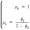
(V.I.1-111)

where (due to (V.I.1-108))

(V.I.1-112)

are starting values of the difference equation.

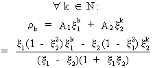
In general, the solution to the difference equation is, according to Box and Jenkins (1976), given by

(V.I.1-113)

In particular, three different cases can be worked out for the solutions of the difference equation

(V.I.1-114)

of (V.I.1-102). The general solution of eq. (V.I.1-113) can be written in the form

(V.I.1-115)

(V.I.1-116)

Remark that for the case the following stationarity conditions

(V.I.1-117)

(V.I.1-118)

has two solutions

due to (V.I.1-114) and

due to

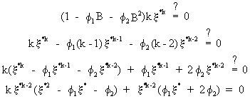
(V.I.1-119)

Hence we find the general solution to the difference equation

(V.I.1-120)

In order to impose convergence the following must hold

(V.I.1-121)

Hence two conditions have to be satisfied

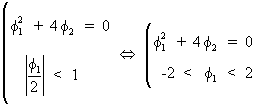
(V.I.1-122)

which describes a part of a parabola consisting of acceptable parameter values for

Remark that this parabola is the frontier between acceptable real-valued and acceptable complex roots (cfr. Triangle of Stralkowski).

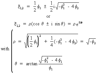
(V.I.1-123)

in goniometric notation.

The general solution for the second-order difference equation can be found by

(V.I.1-124)

On defining

(V.I.1-125)

the ACF can be shown to be real-valued since

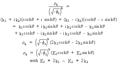
(V.I.1-126)

On using the property

(V.I.1-127)

eq. (V.I.1-126) becomes

(V.I.1-128)

with

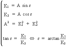
(V.I.1-129)

In eq. (V.I.1-128) it is shown that the ACF is oscillating with period à = 2p/q and a variable amplitude of

(V.I.1-130)

as a function of k.

A useful equation can be found to compute the period of the pseudo-periodic behavior of the time series as

(V.I.1-131)

which must satisfy the convergence condition (c.q. the amplitude is exponentially decreasing)

(V.I.1-132)

The pattern of the theoretical PACF can be deduced from relations (V.I.1-25) - (V.I.1-28).

The theoretical ACF and PACF are illustrated below. Figure (V.I.1-2) contains two possible ACF and PACF patterns for real roots while figure (V.I.1-3) shows the ACF and PACF patterns when the roots are complex.

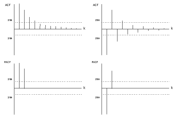
(figure V.I.1-2)

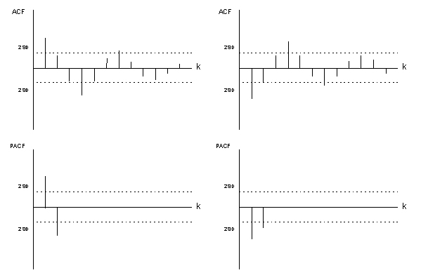
(figure V.I.1-3)