Time Series Analysis - ARIMA models - Basic Definitions and Theorems about ARIMA models

V.I.1.a Basic Definitions and Theorems about ARIMA models

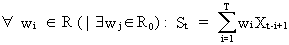
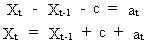
First we define some important concepts. A stochastic process (c.q. probabilistic process) is defined by a T-dimensional distribution function.

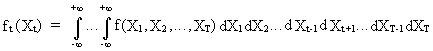
(V.I.1-1)

Before analyzing the structure of a time series model one must make sure that the time series are stationary with respect to the variance and with respect to the mean. First, we will assume statistical stationarity of all time series (later on, this restriction will be relaxed).

Statistical stationarity of a time series implies that the marginal probability distribution is time-independent which means that:

the expected values and variances are constant

(V.I.1-2)

where T is the number of observations in the time series;

the autocovariances (and autocorrelations) must be constant

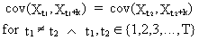
(V.I.1-3)

where k is an integer time-lag;

the variable has a joint normal distribution f(X1, X2, ..., XT) with marginal normal distribution in each dimension

(V.I.1-4)

If only this last condition is not met, we denote this by weak stationarity.

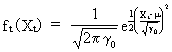
Now it is possible to define white noise as a stochastic process (which is statistically stationary) defined by a marginal distribution function (V.I.1-1), where all X_t are independent variables (with zero covariances), with a joint normal distribution f(X₁, X₂, ..., X_T), and with

(V.I.1-5)

It is obvious from this definition that for any white noise process the probability function can be written as

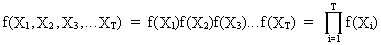
(V.I.1-6)

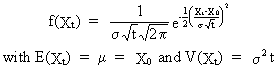
Define the autocovariance as

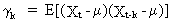
(V.I.1-7)

or

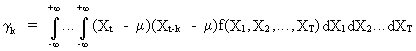
(V.I.1-8)

whereas the autocorrelation is defined as

(V.I.1-9)

In practice however, we only have the sample observations at our disposal. Therefore we use the sample autocorrelations

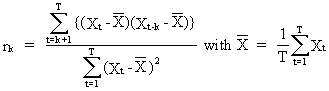
(V.I.1-10)

for any integer k.

Remark that the autocovariance matrix and autocorrelation matrix associated with a stochastic stationary process

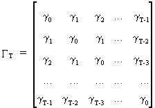
(V.I.1-11)

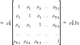
(V.I.1-12)

is always positive definite, which can be easily shown since a linear combination of the stochastic variable

(V.I.1-13)

has a variance of

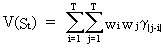
(V.I.1-14)

which is always positive.

This implies for instance for T=3 that

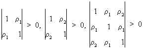
(V.I.1-15)

or

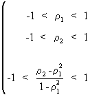
(V.I.1-16)

Bartlett proved that the variance of autocorrelation of a stationary normal stochastic process can be formulated as

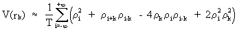
(V.I.1-17)

This expression can be shown to be reduced to

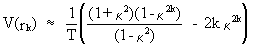
(V.I.1-18)

if the autocorrelation coefficients decrease exponentially like

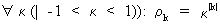
(V.I.1-19)

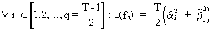
Since the autocorrelations for i > q (a natural number) are equal to zero, expression (V.I.1-17) can be shown to be reformulated as

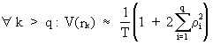
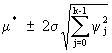
(V.I.1-20)

which is the so called large-lag variance. Now it is possible to vary q from 1 to any desired integer number of autocorrelations, replace the theoretical correlations by their sample estimates, and compute the square root of (V.I.1-20) to find the standard deviation of the sample autocorrelation.

Note that the standard deviation of one autocorrelation coefficient is almost always approximated by

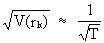
(V.I.1-21)

The covariances between autocorrelation coefficients have also been deduced by Bartlett

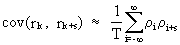
(V.I.1-22)

which is a good indicator for dependencies between autocorrelations. Remind therefore that inter-correlated autocorrelations can seriously distort the picture of the autocorrelation function (ACF c.q. autocorrelations as a function of a time-lag).

It is however possible to remove the intervening correlations between X_t and X_t-k by defining a partial autocorrelation function (PACF)

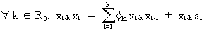
The partial autocorrelation coefficients are defined as the last coefficient of a partial autoregression equation of order k

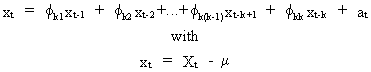
(V.I.1-23)

It is obvious that there exists a relationship between the PACF and the ACF since (V.I.1-23) can be rewritten as

(V.I.1-24)

or (on taking expectations and dividing by the variance)

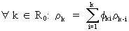
(V.I.1-25)

Sometimes (V.I.1-25) is written in matrix formulation according to the Yule-Walker relations

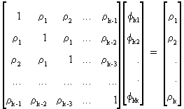
(V.I.1-26)

or simply

(V.I.1-27)

Solving (V.I.1-27) according to Cramer's Rule yields

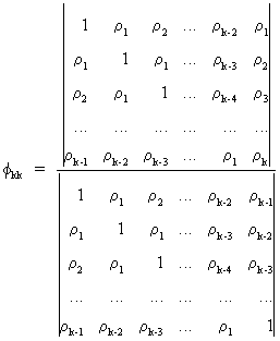
(V.I.1-28)

Note that the determinant of the numerator contains the same elements as the determinant of the denominator, except for the last column that has been replaced.

A practical numerical estimation algorithm for the PACF is given by Durbin

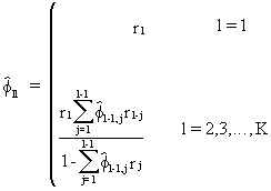
(V.I.1-29)

with

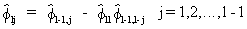
(V.I.1-30)

The standard error of a partial autocorrelation coefficient for k > p (where p is the order of the autoregressive data generating process; see later) is given by

(V.I.1-31)

Finally, we define the following polynomial lag-processes

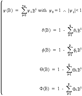
(V.I.1-32)

where B is the backshift operator (c.q. BⁱY_t = Y_t-i) and where

(V.I.1-33)

These polynomial expressions are used to define linear filters. By definition a linear filter

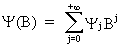
(V.I.1-34)

generates a stochastic process

(V.I.1-35)

where a_t is a white noise variable.

(V.I.1-36)

for which the following is obvious

(V.I.1-37)

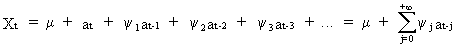
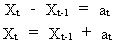
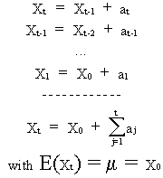
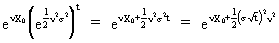
We call eq. (V.I.1-36) the random-walk model: a model that describes time series that are fluctuating around X₀ in the short and in the long run (since a_t is white noise).

It is interesting to note that a random-walk is normally distributed. This can be proved by using the definition of white noise and computing the moment generating function of the random-walk

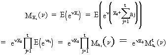
(V.I.1-38)

(V.I.1-39)

from which we deduce

(V.I.1-40)

(Q.E.D.).

A deterministic trend is generated by a random-walk model with an added constant

(V.I.1-41)

The trend can be illustrated by re-expressing (V.I.1-41) as

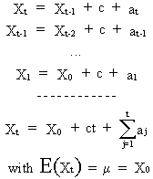
(V.I.1-42)

where ct is a linear deterministic trend (as a function of time).

The linear filter (V.I.1-35) is normally distributed with

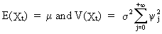
(V.I.1-43)

due to the additivity property of eq. (I.III-33), (I.III-34), and (I.III-35) applied to a_t.

Now the autocorrelation of a linear filter can be quite easily computed as

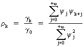
(V.I.1-44)

since

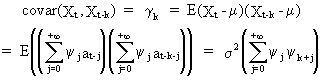
(V.I.1-45)

and

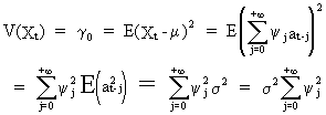
(V.I.1-46)

Now it is quite evident that, if the linear filter (V.I.1-35) generates the variable X_t, then X_t is a stationary stochastic process ((V.I.1-1) - (V.I.1-3)) defined by a normal distribution (V.I.1-4) (and therefore strongly stationary), and a autocovariance function (V.I.1-45) which is only dependent on the time-lag k.

The set of equations resulting from a linear filter (V.I.1-35) with ACF (V.I.1-44) are sometimes called stochastic difference equations. These stochastic difference equations can be used in practice to forecast (economic) time series. The forecasting function is given by

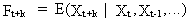
(V.I.1-47)

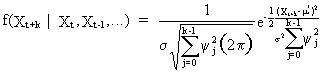
On using (V.I.1-35), the density of the forecasting function (V.I.1-47) is

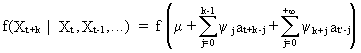
(V.I.1-48)

where

(V.I.1-49)

is known, and therefore equal to a constant term. Therefore it is obvious that

(V.I.1-50)

(V.I.1-51)

The concepts defined and described above are all time-related. This implies for instance that autocorrelations are defined as a function of time. Historically, this time-domain viewpoint is preceded by the frequency-domain viewpoint where it is assumed that time series consist of sine and cosine waves at different frequencies.

In practice there are both advantages and disadvantages to both viewpoints. Nevertheless, both should be seen as complementary to each other.

(V.I.1-52)

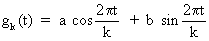
for the Fourier series model

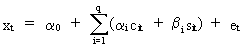
(V.I.1-53)

In (V.I.1-53) we define

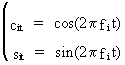
(V.I.1-54)

The least squares estimates of the parameters in (V.I.1-52) are computed by

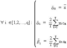
(V.I.1-55)

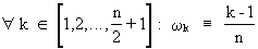
In case of a time series with an even number of observations T = 2 q the same definitions are applicable except for

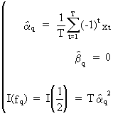
(V.I.1-56)

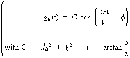
It can furthermore be shown that

(V.I.1-57)

(V.I.1-58)

such that

(V.I.1-59)

(V.I.1-60)

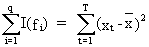
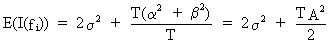
Obviously

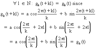
(V.I.1-61)

It is also possible to show that

(V.I.1-62)

If

(V.I.1-63)

then

(V.I.1-64)

and

(V.I.1-65)

and

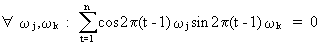
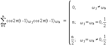
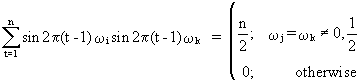
(V.I.1-66)

and

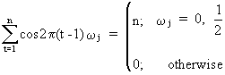
(V.I.1-67)

and

(V.I.1-68)

which state the orthogonality properties of sinusoids and which can be proved. Remark that (V.I.1-67) is a special case of (V.I.1-64) and (V.I.1-68) is a special case of (V.I.1-66). Particularly eq. (V.I.1-66) is interesting for our discussion in regard to (V.I.1-60) and (V.I.1-53), since it states that sinusoids are independent.

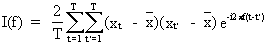
If (V.I.1-52) is redefined as

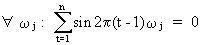
(V.I.1-69)

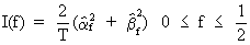
then I(f) is called the sample spectrum.

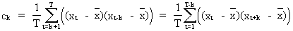
The sample spectrum is in fact a Fourier cosine transformation of the autocovariance function estimate. Denote the covariance-estimate of (V.I.1-7)by the sample-covariance (c.q. the numerator of (V.I.1-10)), the complex number i, and the frequency by f, then

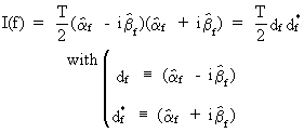
(V.I.1-70)

On using (V.I.1-55)and (V.I.1-70) it follows that

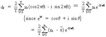
(V.I.1-71)

which can be substituted into (V.I.1-70) yielding

(V.I.1-72)

Now from (V.I.1-10) it follows

(V.I.1-73)

and if (t - t') is substituted by k then (V.I.1-72) becomes

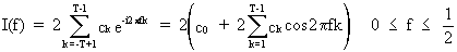
(V.I.1-74)

which proves the link between the sample spectrum and the estimated autocovariance function.

On taking expectations of the spectrum we obtain

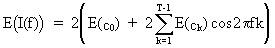
(V.I.1-75)

for which it can be shown that

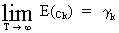
(V.I.1-76)

On combining (V.I.1-75) and (V.I1.1-76) and on defining the power spectrum as p(f) we find

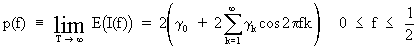
(V.I.1-77)

It is quite obvious that

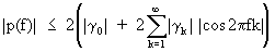
(V.I.1-78)

so that it follows that the power spectrum converges if the covariance decreases rather quickly. The power spectrum is a Fourier cosine transformation of the (population) autocovariance function. This implies that for any theoretical autocovariance function (cfr. the following sections) a respective theoretical power spectrum can be formulated.

Of course the power spectrum can be reformulated with respect to autocorrelations in stead of autocovariances

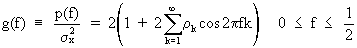
(V.I.1-79)

which is the so-called spectral density function.

Since

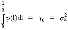
(V.I.1-80)

it follows that

(V.I.1-81)

and since g(f) > 0 the properties of g(f) are quite similar to those of a frequency distribution function.

Since it can be shown that the sample spectrum fluctuates wildly around the theoretical power spectrum a modified (c.q. smoothed) estimate of the power spectrum is suggested as

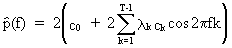
(V.I.1-82)