|
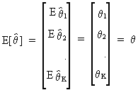
The property of unbiasedness
(for an estimator of theta) is defined by
(I.VI-1)
where the biasvector
delta can be written as

(I.VI-2)
and the precision
vector as

(I.VI-3)
which
is a positive definite symmetric K by K matrix.
If two different estimators of the
same parameter exist one can compute the difference between their
precision vectors: if this vector is positive semi definite this
means we know that the second estimator has a "smaller"
covariance matrix and can therefore be called better
than the first estimator.
An estimator is said to be efficient if it is unbiased and at the same the time no other
estimator exists with a lower covariance matrix.
If Y is a random variable
of independent observations with a probability distribution f then
the joint distribution can be written as

(I.VI-4)
The function of the unknown
parameter, as a function of the values of the random variable, is
called the likelihood
function which has the same structure as the joint probability
function but is dependent on the random variable in stead of the
unknown parameter.
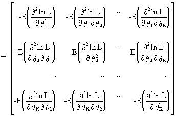
The information
matrix is defined as the negative of the expected value of the
Hessian matrix of the log likelihood function L

(I.VI-5)
(I.VI-6)
The Cramér-Rao
lower bound is defined as the inverse of the information matrix

(I.VI-7)
here
denoted omega.
If an estimator is unbiased
then

(I.VI-8)
is
a positive semi definite matrix. Expression (I.VI-6) is called the Cramér-Rao
inequality.
Proof of this inequality
can be easily obtained. If we consider only one parameter, by
definition of the likelihood function we may write

(I.VI-9)
which can be derived with
respect to the parameter

(I.VI-10)
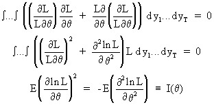
Deriving a second time
yields
(I.VI-11)
This implies that E((D ln L)2)
= - E(D2 ln L) which is equivalent to the information
matrix.
If the estimator is
unbiased then

(I.VI-12)
It follows from (I.VI-10)
that

(I.VI-13)
On combining (I.VI-13) with
(I.VI-12) and applying the Cauchy-Schwarz inequality we obtain

(I.VI-14)
from
which the Cramér-Rao inequality follows immediately.
Note that according to the
Cramér-Rao lower bound

(I.VI-15)
but
not vice versa. This is because the Cramér-Rao lower bound is not
always attainable (for unbiased estimators).
The property of sufficiency
can be formulated as

(I.VI-16)
while the property of consistency is defined as

(I.VI-17)
where
delta is a small scalar and epsilon is a vector containing elements
with "small" values.
The large sample properties
apply only when the number of observations converges towards
infinity in the limit. Accordingly, we can define the large
sample consistency as

(I.VI-18)
where
epsilon is "small".
By definition we can also
use a shorter notation

(I.VI-19)
were
"plim" is the so-called "probability limit". In
this case we say that the estimator for theta converges
in probability to the population value of theta.
A short example will
clarify the concept of large sample consistency. Let us take the
sample mean as an estimator of the population mean. Then it is
possible to prove large sample consistency on using eq. (I.III-47)
applied to the sample mean:

(I.VI-20)
The standard deviation of
the sample mean is known to be

(I.VI-21)
On combining (I.VI-20) and
(I.VI-21) we obtain

(I.VI-22)

(I.VI-23)
Now it obvious that

(I.VI-24)
where the RHS can be made
arbitrarily close to 1 by increasing T (the number of sample
observations). Now we may conclude

(I.VI-25)
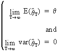
A sufficient, but not
necessary, condition for large
sample efficiency is
(I.VI-26)
According to Slutsky's
theorem the following holds

(I.VI-27)

(I.VI-28)
Other
properties of plims are

(I.VI-29)
and

(I.VI-30)
(this
is true even if both estimators are dependent on each other: this is
not so with the mathematical expectation) and finally

(I.VI-31)
where
AT is a square
parameter matrix.
Note the following
definition of asymptotically distributed parameter vectors

(I.VI-32)

(I.VI-33)
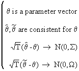
The concept of asymptotic
efficiency can be used to compare
estimators. Formally this is written:
if
(I.VI-34)
then

(I.VI-35)
Finally we describe Cramér's theorem because it enables us to combine plims with
convergence in distribution. Formally this theorem states that if
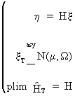
(I.VI-36)

then

(I.VI-37)
| 
