|
In
simultaneous equation systems there are always feedback structures
which make it (almost) impossible to use the easy methods we've
described before.
As a
matter of fact we have to make a firm distinction between two
different kinds of variables: the jointly dependent variables (or
endogenous variables), and the predetermined variables (or exogenous
variables).
The
jointly dependent variables may (but don't have to) be used as
dependent and explanatory variables at the same time (in different
equations). The predetermined variables however are all of those
which are not explicitly explained by other variables in any
equation. This means that a "lagged" version of a
dependent variable is in fact considered to be exogenous or rather predetermined.
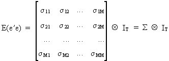
The
variance-covariance matrix
of the residuals is assumed to be of the form
(III.III-1)

The
model of the structural
equations can be written as

(III.III-2)


(III.III-3)
which
leads to

(III.III-4)
and
thus to

(III.III-5)
in
order to get the reduced form
equations.
Remark
that

(III.III-6)
which
are called the reduced form
parameters and the reduced form disturbance respectively.
In
fact, by transforming a structural form into a reduced form, what
one does is to express all jointly dependent variables as a function
of all predetermined variables.
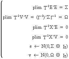
The
asymptotic assumptions
are expressed explicitly as
(III.III-7)
Since
it is our objective to estimate the structural parameters of (III.III-2)
we could start naively with OLS estimations to each equation
separately (after having normalized the equations)

(III.III-8)

Except
in rare cases this procedure will not yield unbiased parameter
estimations since

(III.III-9)

Above
that, the estimated value of the parameters does not converge in
probability

(III.III-10)
The
results in (III.III-9) and (III.III-10) are known as the least squares bias. It is therefore quite obvious that we have to
find other ways of estimating the structural parameters, without
bias.
We
know that estimating the reduced
form with OLS would
be at least consistent
since the assumptions of (III.III-7) can be used to prove that

(III.III-11)
The
OLS estimator will also be unbiased (for estimating the reduced form
parameters) if X doesn't
contain lagged jointly dependent variables.
Suppose
we use (III.III-11) in the context of SUR then we know that this is
equivalent to GLS since all the exogenous variables are identical in
all equations.
After
having used OLS with SUR it is sometimes possible to compute the
structural form parameters knowing that

(III.III-12)

This
procedure is known as the Indirect
Least Squares method (ILS).
When
is it possible to find a unique solution with ILS? Answer: only when
the equations are exactly
identified. If an equation is under identified it is never
possible to compute the structural parameters. If however an
equation is over identified there are more than one unique solution
to (III.III-12), and consequently some special techniques should be
used to solve this problem.
Let
us have a look at the i-th equation of a structural form

(III.III-13)
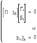
Since

(III.III-14)
we
know that
(III.III-15)
A
necessary and sufficient condition for exact identification is

(III.III-16)
which
is called the rank condition.
Here ILS is consistent and efficient.
A
condition for over
identification is

(III.III-17)
where
ILS is consistent but not efficient.
A
condition for under
identification is

(III.III-18)
where
estimation with ILS is not possible.
A
necessary condition for identification is therefore

(III.III-19)

Now
we consider the problem of estimating the structural parameters of
an over identified system by use of
 | the
ILS approach | |
 | the
GLS approach | |
The
ILS approach
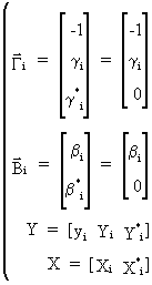
A
single-equation structural form

(III.III-20)
with
(III.III-21)
can
be written as
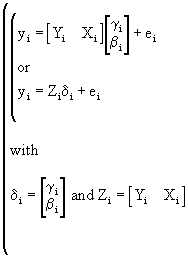
(III.III-22)
Since
the reduced form parameters may be consistently estimated by

(III.III-23)
and
since
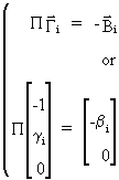
(III.III-24)
it
follows that

(III.III-25)
and
by premultiplying by X'X
we get

(III.III-26)
and
thus

(III.III-27)


(III.III-28)

The
GLS approach
When
the model

(III.III-29)
is
premultiplied by X' we
obtain

(III.III-30)
It
can easily be shown, using (III.III-30), that the GLS estimator is

(III.III-31)
or

(III.III-32)

To
prove consistency, assume

(III.III-33)
which
can be used to show that

(III.III-34)
The
consistent Two Stage Least
Squares estimator (2SLS) consists of the following two stages
first
stage

(III.III-35)
second
stage
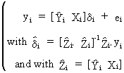
(III.III-36)
Asymptotically
efficient estimators
All
the previous estimators are not efficient (in general) since they
don't use the information to the full extent. Therefore we describe
two Full Information methods: the Tree
Stage Least Squares (3SLS), and the Full
Information Maximum Likelihood Estimation (FIMLE).
The
3SLS estimator uses the following model
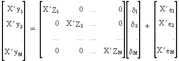
(III.III-37)
or
simply
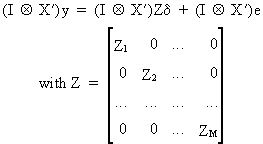
(III.III-38)
If
X'X/T converges to a nonstochastic limit then

(III.III-39)
and
accordingly the 3SLS estimator can be deduced as

(III.III-40)

If
all M equations are identified, the 3SLS estimator is consistent.
Above this, the 3SLS method is more efficient than the 2SLS method.
The
FIMLE method can be used under the assumption that the distribution
of the error terms is known (e.g. normal).
Assume
that the errors are jointly normally distributed with a zero mean
and covariance matrix

(III.III-41)
then
the FIMLE method can be applied by means of for instance a numerical
iterative algorithm. Some examples of algorithms are: the Grid
search method, the Newton-Raphson method, the Gauss-Newton method,
the Steepest Descend method, the Marquardt algorithm etc... | 
