Statistical Inference with Ordinary Least Squares

II.I.4 Statistical inference with Ordinary Least Squares (OLS)

a. Mathematical expectation and variance of parameters

In order to be able to say something about the population parameters (of the real mathematical model), based only on the sample observations, it is imperative to compute the expectation and the variance of both estimated parameters.

The expectation of the estimated constant term can be derived as follows

(II.I.4-1)

(II.I.4-2)

It is quite easy to derive the variance of the constant term as

(II.I.4-3)

Now consider the derivation of the expectation of the estimated ß parameter

(II.I.4-4)

(II.I.4-5)

(II.I.4-6)

The derivation of the variance is quite similar to (II.I.4-4)

(II.I.4-7)

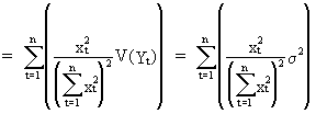
(II.I.4-8)

(II.I.4-9)

From this analysis we conclude that in order to reduce the variance of the estimated parameters we should ensure that:

	(a) the number of sample data should be large because of eq. (II.I.4-3);
	(b) the (constant) variance of the endogenous variable should be relatively small (see eq. (II.I.4-3) and eq. (II.I.4-9));
	(c) the range of the exogenous variable should be large because of eq. (II.I.4-9).

Remark that (a) and (c) is not only true in simple regression but also in all other econometric regressions (time series and cross-sectional data), multivariate statistic techniques, statistic time series analyses, random experiments, and even in controlled experiments (this only applies to (c) ).

Furthermore, it can be concluded from eq. (II.I.4-2)and eq. (II.I.4-6)that OLS for simple regression yields unbiased estimates for both parameters.

b. Confidence intervals for the parameters

In order to find the t statistic we first derive the Z transformation of the estimated value of ß

(II.I.4-10)

where the unobservable s is replaced by the sample variance since

(II.I.4-11)

so that by definition

(II.I.4-12)

Furthermore, the 95% confidence interval for any ß parameter is given by

(II.I.4-13)

(II.I.4-14)

where

represents the limit value of ß according to the students t-distribution (for the 5% significance level).

The confidence interval for a can be found in just the same way (cfr. (II.I.4-10) to (II.I.4-14)).

c. Forecasting errors

If the mean forecast is considered, a suitable confidence interval should be derived.

First we note

(II.I.4-15)

(we say: the mean estimator (II.I.4-15) is unbiased).

Additionally, the expression for the variance of the mean estimator is found as

(II.I.4-16)

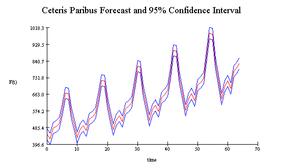
Example of interpolation confidence interval

It is obvious from (II.I.4-16) that the forecast performance depends on: the variance of the endogenous variable, the sample size, the range of the exogenous variable, and x₀; the distance between the forecast origin and the mean of the exogenous variable.

If however, an individual estimation of Y at origin t = o (o = origin) has to be performed, the variance should be added to (II.I.4-16)

(II.I.4-17)