Online Econometrics Textbook - Regression Extensions - Finite distributed lags

III.VI.1 Finite distributed lags

We define finite distributed lags by the following underlying model

(III.VI.1-1)

where K is the (finite) number of lags to be considered. Apparently, estimation of (III.VI.1-1) for K smaller than T is easily obtained by the OLS estimator which is, under OLS assumptions, BLUE.

Remark however that in practice estimation of (III.VI.1-1) might become difficult due to the possibility of multicollinearity (due to high autocorrelation in X).

Also note that in this model K is assumed to be known. If this parameter is not specified correctly the existence of an Unobserved Variables Bias is quite realistic. Therefore a selection criterion is often used to specify the lag length. One of the most popular criteria is the Akaike Information Criterion (AIC)

(III.VI.1-2)

where sigma is the maximum likelihood estimator for the variance (cfr. (II.II.2-7)). The AIC criterion must be minimized to find the optimal model structure.

Remark however that all selection criteria found in the econometrics literature should be used with great care! According to Judge et al. : "Although there is a certain intuitive appeal and logic to many of the ad hoc, informal model selection rules that have been suggested, we should not forget (1) their heuristic base, (2) the fact that their sampling properties are virtually unknown, and (3) that their practical utility is mainly demonstrated by numerical examples." (Judge et al. 1985, p. 888).

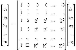
When it is assumed that the b coefficients are polynomially distributed according to a finite time lag, we call these Almon lags. Finite polynomially distributed lags of order Q can be written as

(III.VI.1-3)

Obviously, a shorter description of (III.VI.1-3) is

(III.VI.1-4)

(III.VI.1-5)

it follows that

(III.VI.1-6)

or (in terms of the original parameters)

(III.VI.1-7)

which is in fact a kind of RLS estimator for the polynomially distributed b parameter vector.

Under OLS assumptions it can be shown that

(III.VI.1-8)

In practice it follows from the above that estimation of Almon lags is quite simple if K and Q are known beforehand. This however is not always the case, moreover there exist a lot of difficulties in identifying K and Q. As mentioned earlier, the ad hoc selection criteria should be used with great care.

Sometimes it is assumed that the regression parameters follow a polynomial spline lag. Formally this is

(III.VI.1-9)

where i_K is the true lag length, and

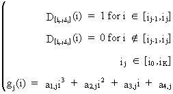
(III.VI.1-10)

In order to obtain a smooth distribution it is necessary to impose the following structure on the cubic polynomials

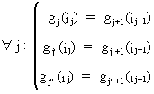
(III.VI.1-11)

Now the same procedure as with the Almon lags is used to derive the polynomial spline lag estimator

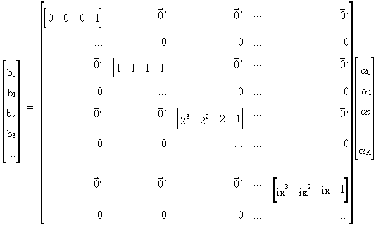
(III.VI.1-12)

with

(III.VI.1-13)

Compactly this can be written like (III.VI.1-4) and the appropriate RLS estimator is analogous to the derivation of the Almon lag estimator.

Last but not least define the harmonic distributed lag as

(III.VI.1-14)

Eq. (III.VI.1-14) becomes (III.VI.1-7) in short notation and

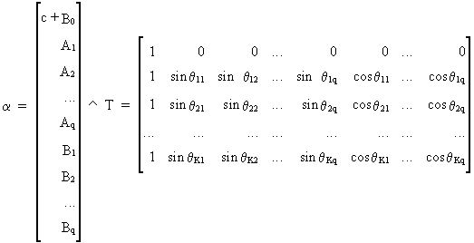
(III.VI.1-15)

Obviously, estimation of these harmonic distributed lags is analogous to the estimation of Almon lags.