III.I.2 Autocorrelation in Linear
Regression
How can we solve the problem of autocorrelation as in (III.I.2-1))?

(III.I.2-1)
We can
write (III.I.2-1) in terms of variances

(III.I.2-2)
but since we may assume homoskedasticity it follows that

(III.I.2-3)
Using
(III.I.2-1) the covariance with a lag of 1 period is

(III.I.2-4)
In general the covariance with lag k can be written as

(III.I.2-5)
and
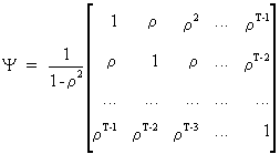
the covariance matrix of the residuals as

(III.I.2-6)
which
therefore yields

(III.I.2-7)
The
GLS solution to this
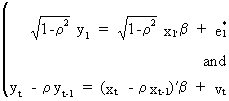
problem, if r is assumed to be known, is a tree stage procedure
stage
1

(III.I.2-8)
stage
2

(III.I.2-9)
stage
3

(III.I.2-10)
using
equation (III.I-8).
Remark
that

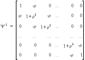
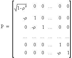
(III.I.2-11)
and
that

(III.I.2-12)
which
implies

(III.I.2-13)

There
are two other alternatives to solve the problem of (III.I.2-1):
lagged variables, and distributed lags.
Sometimes
lagged endogenous and/or
exogenous variables can
be introduced in order to reduce the autocorrelation problem. This
is a quite flexible tool with however, one important drawback. The
introduction of each additional
variable reduces the degrees of freedom, whereas the use of a lagged
variable mostly forces the researcher to reduce the sample range
which also implies a loss of degrees of freedom (º
T - K). Also remember that OLS is not an efficient estimator in the
context of autocorrelation. Even worse is the estimation of
parameters of lagged endogenous variables in the context of
autocorrelation induced by unobserved variables (or wrong
specification): in this case the OLS estimates will be biased.
Distributed
lags can also be used to solve problem of (III.I.2-1).
A huge advantage over the lagged variables method is that the
distributed lags do not incur as large a loss of degrees of freedom
as the first method. A drawback of this method could be the fact
that the estimation procedure is not always straightforward and
sometimes even difficult. The method of distributed lags will be
discussed in detail in later sections.
In
econometrics the Durbin-Watson
statistic (c.q. d statistic) is frequently used

(III.I.2-14)
Since

(III.I.2-15)
eq.
(III.I.2-14) can be rewritten as

(III.I.2-16)
for
large samples, where r
is the correlation between the residual at period t and the residual
at t-1. Note that d = 2 in case there is no (first order)
autocorrelation in the residual series.
The
Durbin-Watson statistic will fail when time series data are strongly
seasonal. In this case an adapted d statistic, for a seasonal period
s, can be defined as

(III.I.2-17)
which
is in fact an autocorrelation coefficient of order s.
The
d statistic will, in general, also fail in case a regression
equation under OLS is estimated with the lagged endogenous variable
variable used as regressor. In this case Durbin suggests
alternatives (the so-called h statistics) such as

(III.I.2-18)

Another
way to detect AR(p) autocorrelation is the Breusch-Godfrey
test based on a test-equation: the residuals are explained by
its lagged values (p is the number of lags included in the
test-equation) and all exogenous variables of the original equation.
The presence of AR(p) autocorrelation is tested by the use of a
Chi-square-statistic (c.q. (T-p)*R-square).
Below
you ll find an example of how the Breusch-Godfrey test can be
applied to test for AR(p) autocorrelation (this test is applied to
our example-equation):
Breusch-Godfrey test for AR(p) residuals by Least Squares:

Estimation with OLS:

Endogenous variable =  Residuals

Variable                     Parameter                S.E.      T-STAT
employ                   -6.574423604           7.235339332     -0.909
expend                   +2.286765988           2.796278607     +0.818
const                   +82.24312207          278.872104        +0.295
resid(-1)                -0.449639967           0.2411178087    -1.86
resid(-2)                -0.2887649456          0.194556882     -1.48
resid(-3)                -5.403469274e-002      0.2080984616    -0.26

2-tail-t at 95 percent = 2.042
1-tail-t at 95 percent = 1.697
R-squared of stationary series = 0.1647233405
Durbin-Watson                  = 1.999045701
Degrees of freedom             = 30
Variance of regression         = 1052262.317
Standard Error of regression   = 1025.79838
Sum of Squared Residuals       = 31567869.52

Correlation matrix of parameters:


            +1.00  -0.91  -0.51  +0.67  -0.08  +0.34
            -0.91  +1.00  +0.21  -0.61  +0.14  -0.27
            -0.51  +0.21  +1.00  -0.31  -0.00  -0.21
            +0.67  -0.61  -0.31  +1.00  +0.16  +0.42
            -0.08  +0.14  -0.00  +0.16  +1.00  +0.20
            +0.34  -0.27  -0.21  +0.42  +0.20  +1.00

(T-p)*R-square =  5.435870235
Critical Chi-square value (95%) = 7.81 (degrees of freedom = 3)
Many
other tests are available to diagnose autocorrelation problems, many
of which belong to the domain of time series analysis (chapter 5). | 
